Comparing Classifier Performance – Introduction to BEA
Published:
Reading time: 10 minutes
Where’d you get the idea, Matt?
I have a nifty program called MIW’s AutoFit that fits 1D data to a variety of functional models. These functional models are built procedurally from a list of primitive functions [sin(x), cos(x), exp(x), log(x), x, 1/x, const] that are combined in standard ways (addition, multiplication, composition). The cool part of this program is that MIW’s AutoFit will test each procedurally-generated functions, and of those tested it will tell you which model is the best for your data.
I was trying to come up with a way to quote a single number for the performance of this program (let’s say for a resumé). It currently has a 100% accuracy with a depth of 1 (6 functional models), a 78% accuracy when the depth is 2 (18 models), 45% accuracy when the depth is 3 (115 models), and a 23% accuracy when the depth is 4 (865 models). Which accuracy do I quote? An accuracy of 100% is deceptive, an accuracy of 23% undersells the power of the program, and quoting many accuracies along with the context is too confusing for an impatient reader.
This got me to thinking: how do you compare the performance of classification algorithms when the number of classes is different? Is a binary classifier with an accuracy of 99.99% actually better than a classifier with an accuracy of 20% across 1000 classes?
Running the Gauntlet
Imagine you’ve built a model that can classify images into 5 categories. When provided with an image, it will output the degree of association$^†$ $\mathbf{D}$ that the image has with each of the 5 categories. It might look something like this
\[\mathbf{D}(\mathrm{image}) = [0.10, 0.05, 0.20, 0.30, 0.35]\]The model associates the image data most strongly with the fifth class ($D_5 > D_{1,2,3,4}$), and therefore the model will classify the image into that category.
Let’s run some hypothetical experiments on this model. Imagine that you run many images from class 5 through the model to find its accuracy $\mathcal{A}_5$ on this category
\[\mathcal{A}_5 = P(D_5 > D_{1,2,3,4} | 5-\mathrm{image}).\]We could also run this same model through a series of parallel experiments, where only two categories are available at a time. If only classes 1 and 5 are available as options, then the accuracy in this scenario is
\[\mathcal{A}_{5,1} = P(D_5 > D_1 | 5-\mathrm{image}),\]and this goes on up to
\[\mathcal{A}_{5,4} = P(D_5 > D_4 | 5-\mathrm{image}).\]We can imagine that when a full 5-category classification is done, it proceeds through a gauntlet of pairwise choices. First the classes 1 and 5 are compared, and if 5 is chosen by the model (with probability $P(5>1|5)$), then the classes 2 and 5 are compared. If class 5 is better pairwise than each of the other classes, then class 5 is chosen as the best overall ($P(5>1,2,3,4|5)$).
Since survival probability is multiplicative, the probability of class 5 making it through the entire gauntlet is equal to the product of probabilities for each of the steps in the gauntlet
\[P(5>1,2,3,4 | 5) = P(5 > 1 | 5) P(5 > 2 | 5) P(5 > 3 | 5) P(5 > 4 | 5)\]If we take the geometric mean of the 4 pairwise probabilities,
\[p_{gm,5} = ^4\sqrt{P(5 > 1 | 5) P(5 > 2 | 5) P(5 > 3 | 5) P(5 > 4 | 5)}\]then we see that the accuracy on 5-class images is
\[\mathcal{A}_5 = p_{gm,5}^4\]I.e. the accuracy on some particular class is equal to the geometric mean of pairwise accuracies, raised to the power of the number of classes less one.
The overall accuracy of the model will be
\[\mathcal{A} = \mathcal{A}_1 P(\mathrm{class\ 1}) + \ldots + \mathcal{A}_5 P(\mathrm{class\ 5})\]where the $P(\mathrm{class\ i})$ simply accounts for the proportion of $i$-class images in the test set. For a perfectly balanced dataset, this reduces to the mean
\[\mathcal{A} = \frac{1}{5}\left[ p_{gm,1}^4 + \ldots + p_{gm,5}^4 \right]\]Remember: we’re trying to find a single number that can be used to compare models with any number of target classes. So when we report this single number, we shouldn’t need to also report the number of classes that the models were tested on. Let’s define the average that appears on the right as
\[\frac{1}{5}\left[ p_{gm,1}^4 + \ldots + p_{gm,5}^4 \right] \equiv \mathcal{A}_{BE}^4\]where the exponent on the right has been chosen to have the same “units” of probability as on the left. This value – \(\mathcal{A}_{BE}\) – is what I call the binary-equivalent accuracy. If I report a certain binary-equivalent accuracy, you can picture that my model will, on average$^‡$, have that level of accuracy when given only two possible options.
So we have a number
\[\mathcal{A}_{BE} = \mathcal{A}^{1/(N-1)},\]but as we shall see in the next section, the asymptotic behaviour of $\mathcal{A}_{BE}$ as the number of classes increases is not entirely satisfactory.
Benchmarking BEAs with Random Guesses
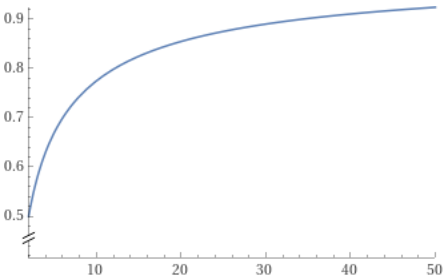
To get a better understanding of what the binary-equivalent accuracy is saying, let’s use a simple toy model to see how the BEA behaves as the number of categories increases. If we have $N$ categories and all our model does is randomly guess the correct category (say with an N-sided die) then its accuracy will be $\mathcal{A}=1/N$, giving a corresponding binary-equivalent accuracy of
\[\tilde{\mathcal{A}}_{BE} = \left(\frac{1}{N}\right)^{1/(N-1)}\] 
The binary-equivalent accuracy (BEA) rises as the number of classes increases. Uhoh! While accuracy as a measure unfairly disadvantages models with a higher number of class labels, the BEA unfairly disadvantages models with fewer categories. In short – the binary-equivalent accuracy of randomly guessing isn’t 50%.
For completeness though, let’s have a look at another model.
Hearing Experiments – A Playground for Testing
Imagine you’ve been asked to participate in an experiment. The researchers sit you down in a quiet room and ask you to indicate whether a sound originated from your left or right side. The sound comes from a random point in the circuar wall that surrounds you. For sounds from your far left or right the task is easy, and you can always identify where the sound is coming from. Your accuracy will be something like 99.5%, with the incorrect trials coming from times where you mixed up the response switches, or the sound bounced funnily in the room, or you were distracted thinking about some funny joke. Alternatively, when the sound is from directly in front of you, but shifted ever so slightly to the left or right, you’re basically just guessing whether the sound was more left or right. There, your accuracy will drop to ~50%. Integrated over all possible sound locations (the 360° around you), your net accuracy might sit around 98%.
Now what happens when they add more options? Left, right, front, back? Or more? Your accuracy will drop, and eventually drop to zero as the number of options increases to infinity, but lets see how the binary-equivalent accuracy behaves in this setting.
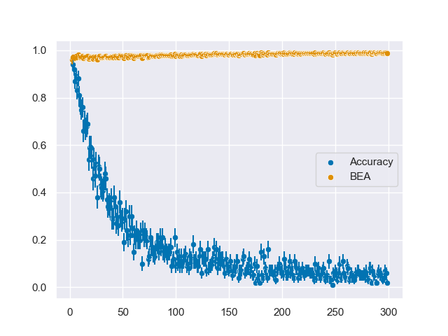
I’ve coded up a simple simulation that can be downloaded here. If a beep comes from an angle $\theta\mathrm{,}$ we pretend that the angle at which you perceive the sound will follow a normal distribution centered on $\theta$ and with some spread $\sigma$. For humans the width of the distribution is about $\sigma \sim 10°$. You point at the perceived source of the beep, and your net accuracy is determined by how often you point in the correct quadrant, hextant, octant, etc. For N categories, the accuracies and binary-equivalent accuracies are shown below

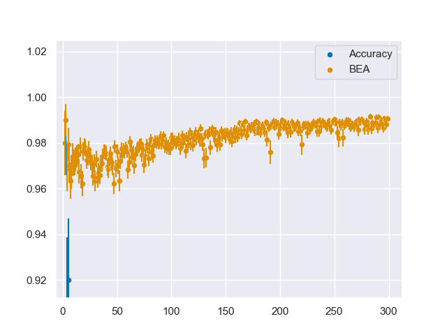
Zooming in on the BEA curve for readability,

we can see that BEA is mostly constant for the first 100 values of $N$, but just like the Random Guess classifier, it slowly grows as $N$ increases. Ideally the profile should be constant, since now one might conclude – based only on the binary-equivalent accuracy – that a human who can distinguish between 100 different categories of angle is better than a human who can only distinguish between 2 different categories of angle – even though they’re the same human!
Despite this obvious drawback, we might as well finish what we started. So let’s take a look at what the Binary-Equivalent Accuracy says about MIW’s AutoFit.
MIW AutoFit’s Binary-Equivalent Accuracy
From the benchmarking accuracies in the introduction of this article, here are their respective binary-equivalent accuracies
| Depth | # Classes | Accuracy | BEA |
|---|---|---|---|
| 1 | 6 | 100% | 100% |
| 2 | 18 | 78% | 98.5% |
| 3 | 115 | 45% | 99.3% |
| 4 | 865 | 23% | 99.8% |
The rising BEA values as the number of classes grows is still apparent here. I would be happy to report that the model has a binary-equivalent accuracy of over 98%, but it would feel disingenuous to report a BEA of 99.8%. More work needs to be done.
Future directions
The rising behaviour of the binary-equivalent accuracy is not entirely optimal, so if and when I find a better idea I’ll update with a new blog post. My current ideas involve either reporting p-values of a certain accuracy relative to the randomly guessing (i.e. what is the probability that a Random Guess classifier would get an accuracy better than the measured accuracy on $N$ classes), or reporting the improvement in wrong-guess instances relative to a Random Guess classifier.
But at the moment I think I’m relatively satisifed with the idea behind BEA: a multiclass classifier can be thought of as a series of binary classifications, and the BEA reports a certain average for the accuracy across each of these binary choices.
$^†$: Despite being the result of a softmax function, and despite being commonly called so, I am hesitant to call this a probability.
$^‡$: The averaging is a certain combination of geometric and arithmetic means.
Tags: #classification #algorithm #statistics #binomial #CDF #binary #equivalent #accuracy
