MIWs AutoFit – Tutorial 5 – Manual Models

Tutorial Sections: 1 2 3 4 5

Now that you’ve made it through the procedural models tutorial, we can discuss constructing our own models.

Okay, great, AutoFit is pretty good with the basic functional building blocks used in most models. But what happens when these building blocks aren’t enough? AutoFit allows you to define functions based on arbitrary Python code, assuming that

1. the code uses no spaces
2. the code you wish to use is base Python, or from the numpy (np) or scipy (scipy.stats or scipy.special) packages

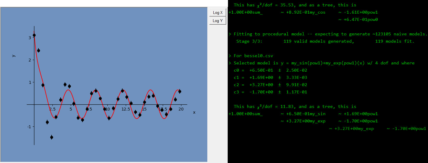
A fairly common function that isn’t considered simple is 0th-order Bessel Function of the first kind, \(J_0(x)\). Loading up a dataset bessel_data.csv⭳ generated with this function, we can first try to fit this function using a combination of exponentials and trigonometric base functions. A reduced chi-squared of 11.83 isn’t too good, and the residuals are decidedly in favour of this model sin(pow1)+exp(pow1) not being the correct function for this dataset.

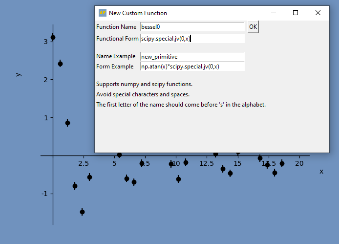
While in Procedural mode, let’s head down to the custom function button in the bottom left of the window. After clicking, we see a pop-up allowing us to create a new base function, which will be included in all subsequent compositions/products/sums when building a list of functional models to test. If we know that the model should be some bessel function of the first kind, implemented using the scipy.stats.jv function, we can declare this as a new base function. Unfortunately AutoFit still is unable to fit two-parameter functions, so the first argument \(\nu\) for jv has to be input by hand.

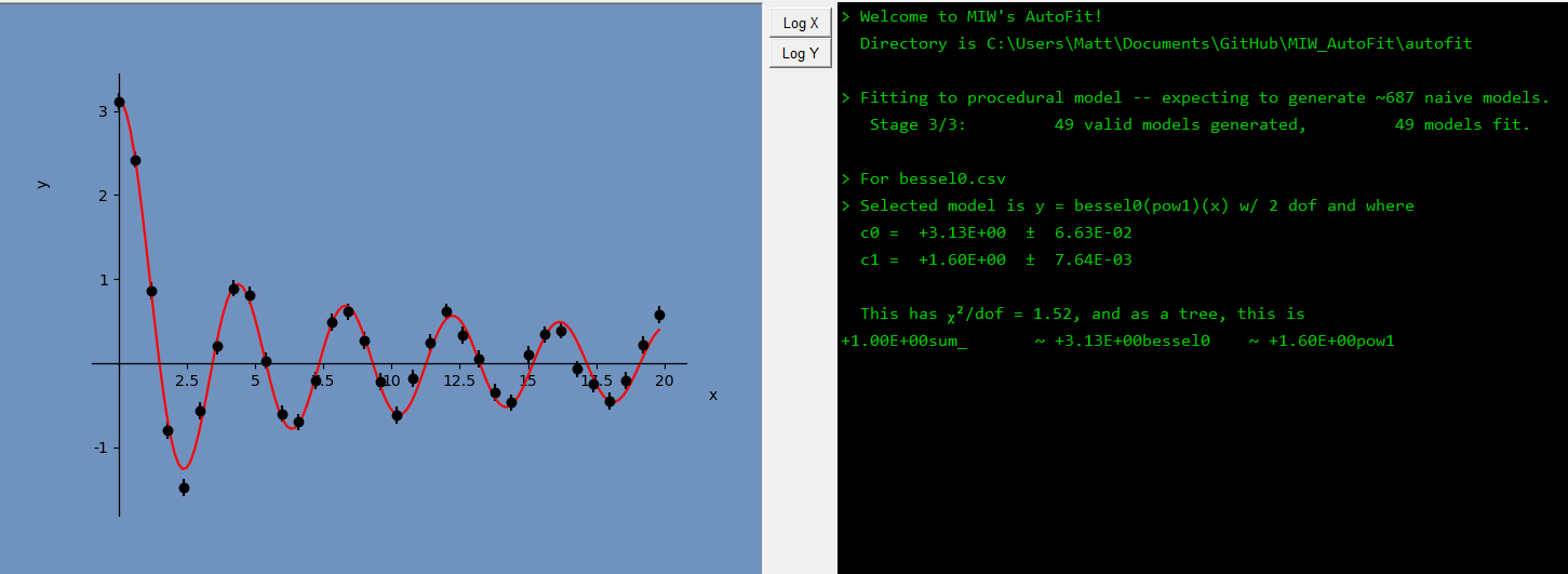
Now when we run the procedural fit for this dataset (ensuring that the custom functions checkbox has a checkmark), we get a good fit for the data

If you would like to remove a custom-made base function from the list of custom functions, you’ll have to navigate to frontend.cfg in your installation directory and manually remove the corresponding entries next to the #CUSTOM_NAMES and #CUSTOM_FORMS tags.

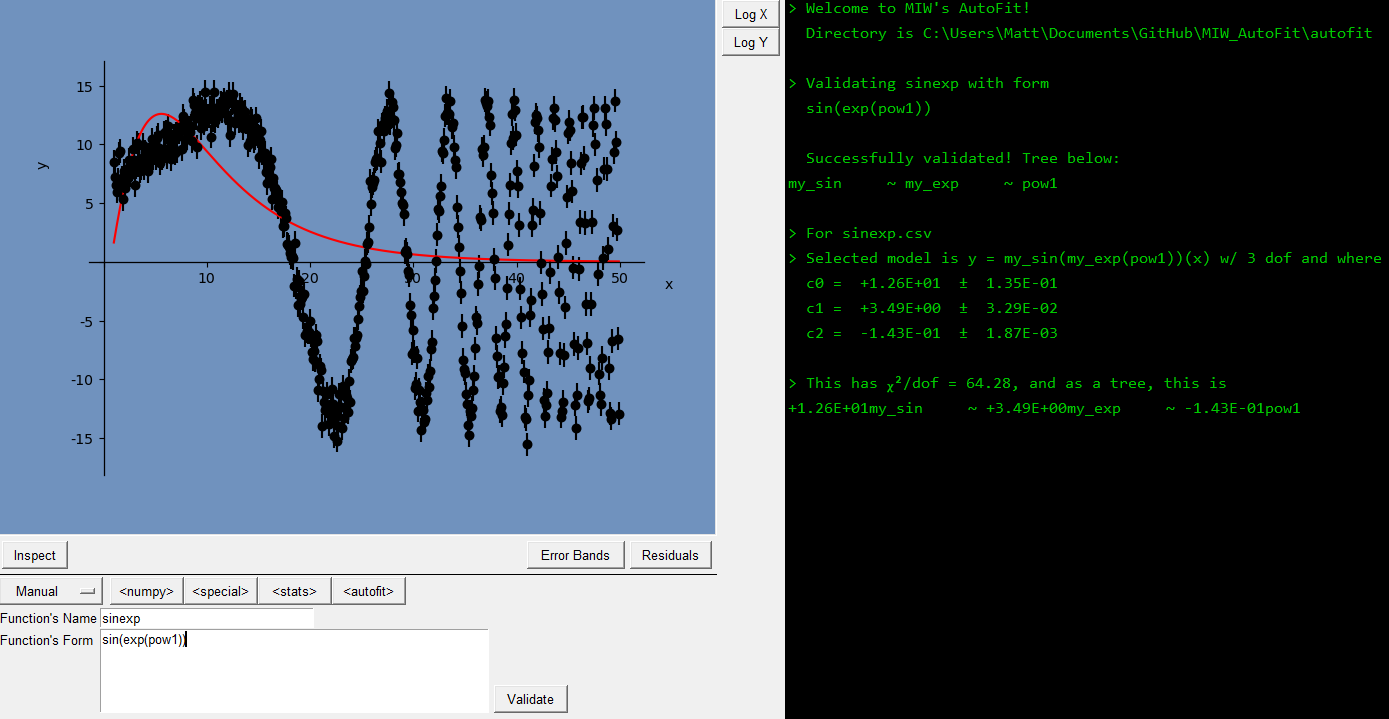
Another issue that might arise is that AutoFit’s search algorithm fails to find a global minimum for a model that actually describes the data very well. Let’s examine the dataset sinexp.csv⭳ generated with the function

AutoFit can’t find the correct fit for this dataset. Let’s try to help it out by going to the Manual dropdown option.

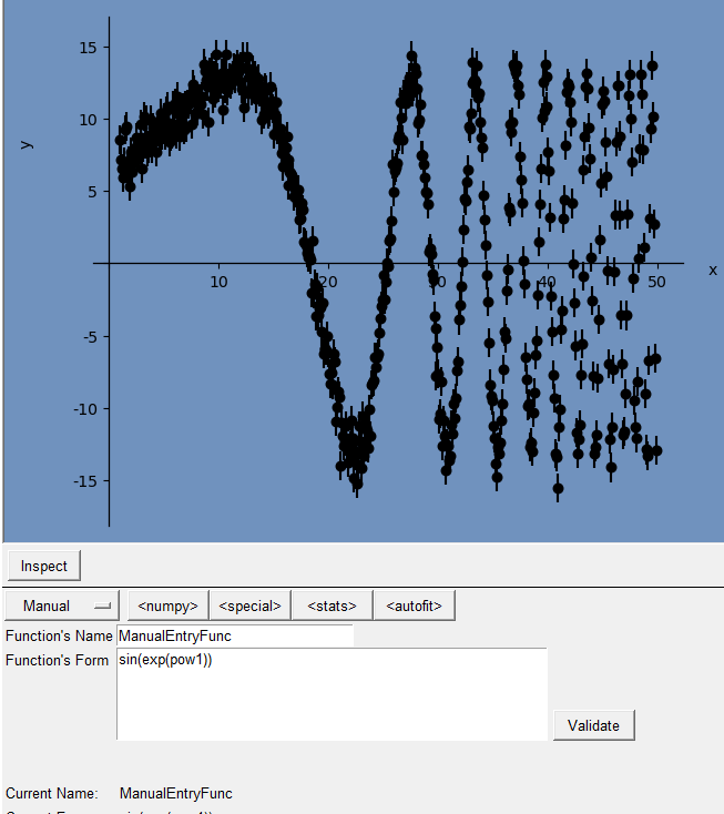
Putting the model into the input field, validating that the input corresponds to a valid function, and clicking Find Fit, we see that AutoFit has found a local minimum for the chi-squared of this model.

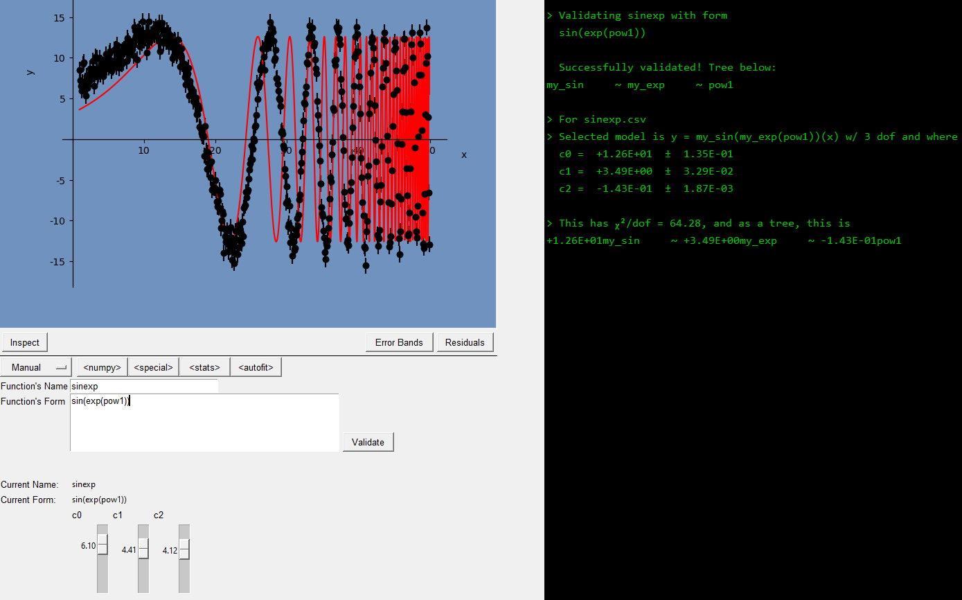
The global minimum can’t be reached from here using its search strategy. But notice that a set of sliders has appeared at the bottom of the window, where we can help it out by adjusting its initial search parameters. Dragging these sliders up and down, we can see how the model would appear with a new set of coefficients (These are in a signed-log scale: Positive slider numbers show \(\log_{10}(arg)+5\), while negative slider numbers corresond to \(-\log_{10}(-arg)-5\)).

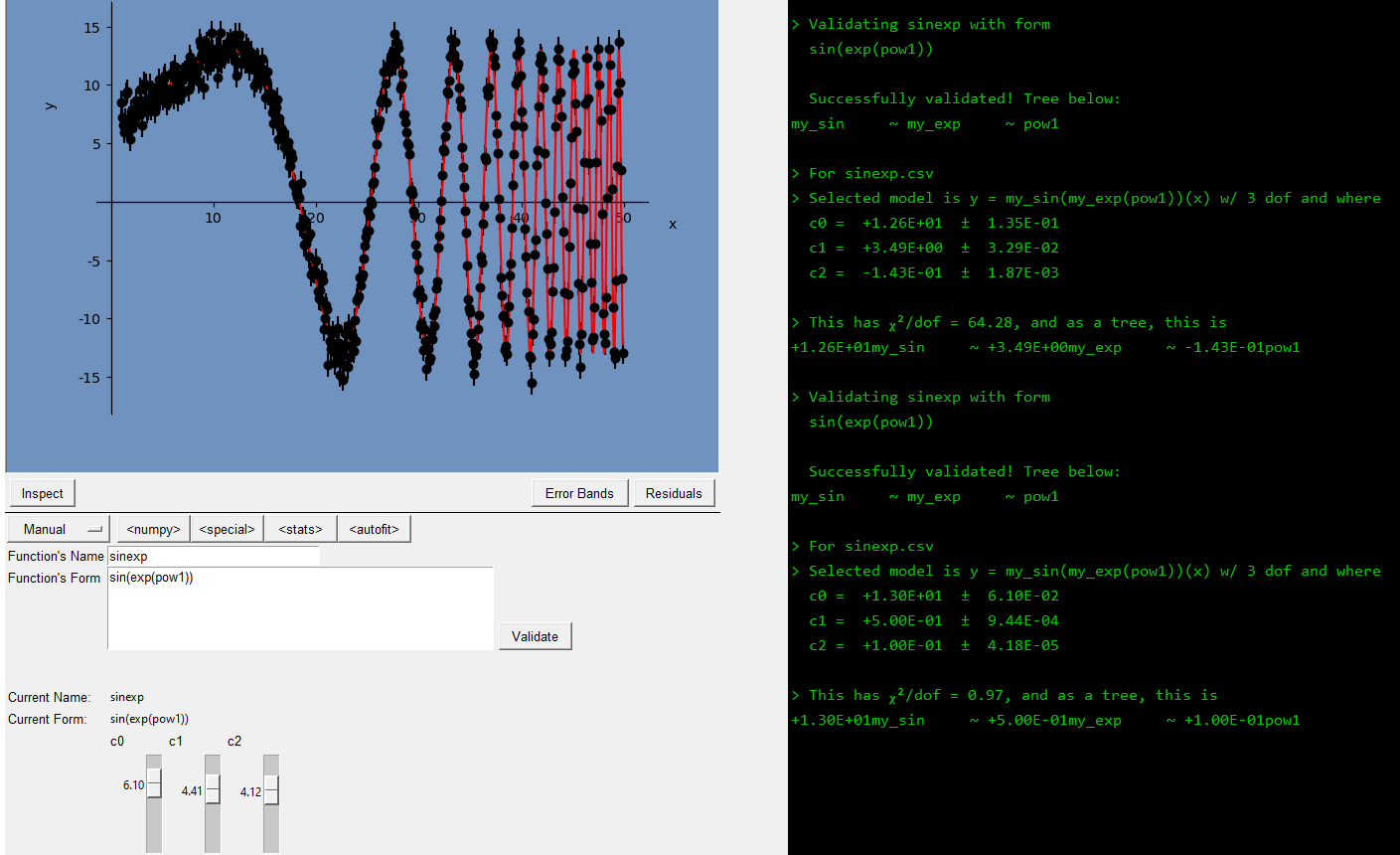
If you can manually find a set of parameters that looks “close enough” to a global optimum,

you can press the “Fit Data” once again to let AutoFit do the rest.

That wraps it up for the tutorials! You’re a pro now, so I wish you luck with all your endeavours!