MIWs AutoFit – Tutorial 4 – Procedural Fits

Tutorial Sections: 1 2 3 4 5

So you’ve made it through the Brute-Forcing tutorial! If you were frustrated with how long the program takes to find a good model, have understood how AutoFit contructs models from base functions, and you would like more control, then this tutorial is for you! In this tutorial we show how to turn off and on certain base functions to create a
more streamlined search in the space of possible models.

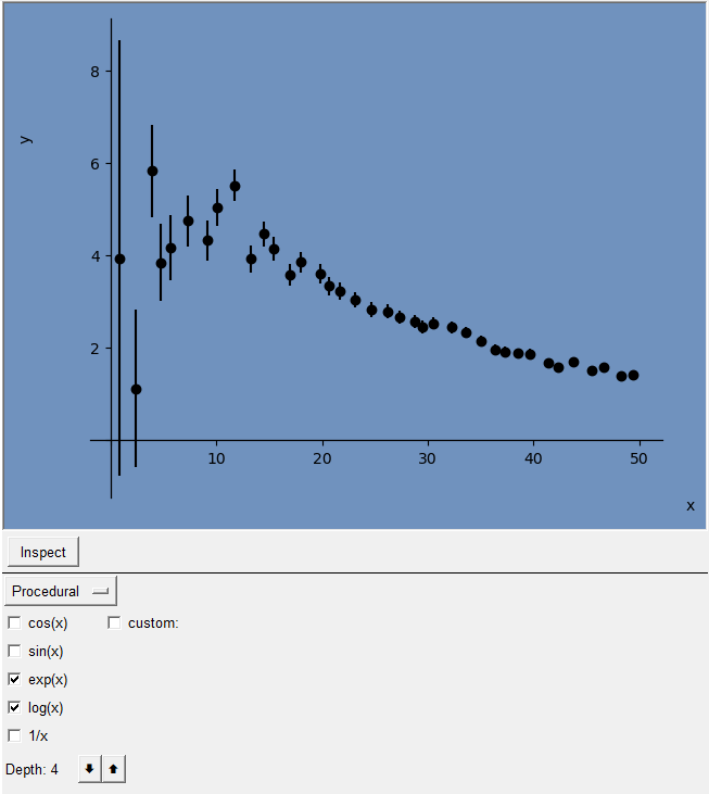
In the last tutorial it took ~40 seconds and 900 model fits to find a good model for the data. Let’s do it again, but with the knowledge that the model only contains exponential and logarithmic functions.

This time, after loading in sudakov.csv⭳ , select the Procedural dropdown option. You will be presented with some checkboxes. Ensure exp and log are selected, and change the depth to 4 (this is the max number of base functions which will be allowed in the generated model list).

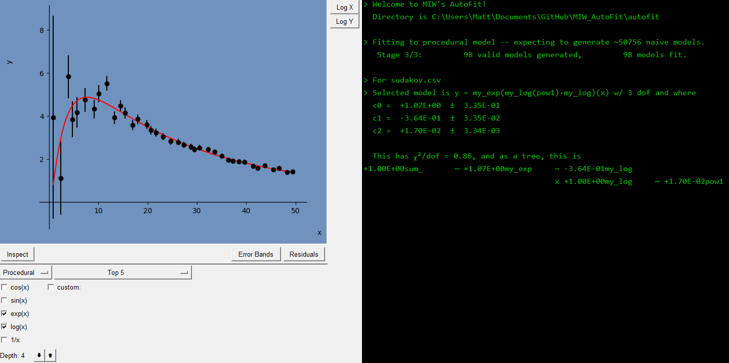
When you click Fit Data, a list of possible models will be created according to the given parameters. This list is then trimmed of invalid models according to various rules (like no exp(exp), or log(log), or sin(cos) – you’ll have to look at the code for the full ruleset), then each model in the trimmed list is fit to the data. In ~7 seconds, we find the same model as in Tutorial 3.

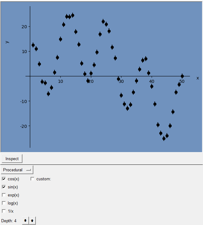
Let’s do another example. Opening sin_cosine.csv⭳ , we see a wavelike structure. Assuming now that there are no logarithmic, exponential, or 1/x base functions, we turn on only sin and cos base functions.

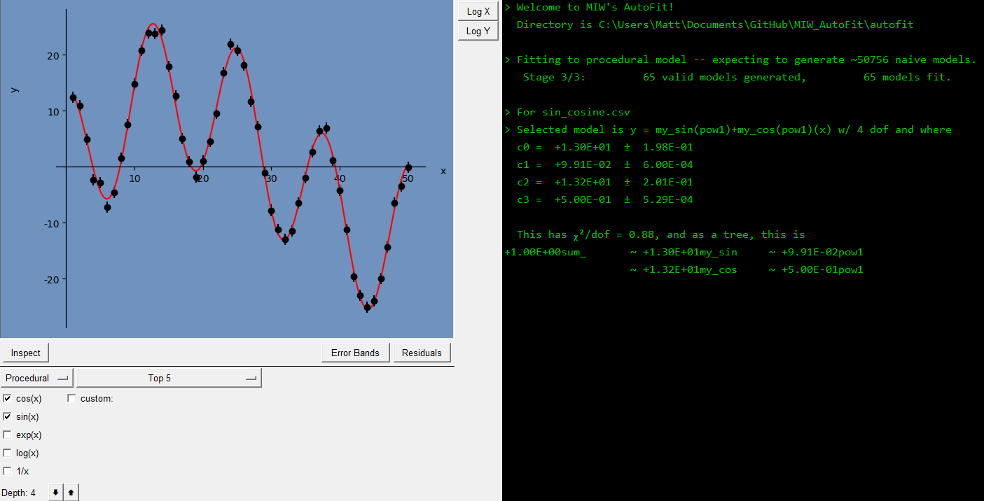
Pressing the Fit Data button, in ~4 seconds we find the correct model that was used to generate the data: a sum of sins and cosines, with different frequencies.

In the final tutorial, we will talk about custom functions – for when AutoFit doesn’t use a particular base function you need – and manual functions, for those cases where MIW’s AutoFit has failed to find the correct model and you know which model it should have found.