MIWs AutoFit – Tutorial 3 – Brute Forcing

Tutorial Sections: 1 2 3 4 5

Hello and welcome to the third tutorial! Today we learn about the most exciting feature of MIW’s AutoFit — finding a fit for a dataset when you don’t know which function your data should follow! In this lesson we learn how to read AutoFit’s internal representation of a function in order to interpret the output of our brute-forcing functionality.

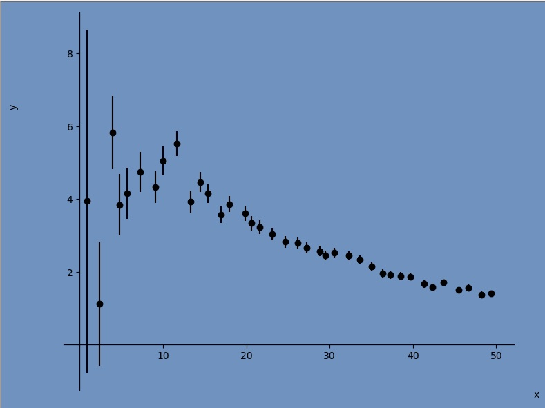
Again, let’s make sure AutoFit has a fresh start so we’re all on the same page. After closing the window, open AutoFit again and load up sudakov.csv⭳ . Head to the dropdown options (if you were following the last tutorial, this should say Gaussian), and choose Brute-Force.

Are you ready? Press Fit Data and watch as MIW’s AutoFit automatically fits your data! It does this by constructing many different functional models and fitting each to the given data. The best five are kept (by default, the reduced chi-squared statistic is used as a discriminating parameter — this can be changed in the settings panel to AIC, AICc, BIC, or HQIC) and the rest are thrown away. After 5 seconds I have hit pause, giving me the output you see below.

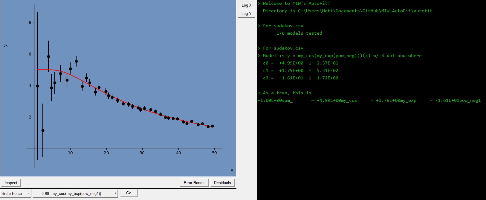
On my machine, AutoFit now believes that the function called my_cos(my_exp(pow_neg1)) is the best function for the dataset. In math, this should read

As you can see, a functional model is made of sums, compositions, and multiplications of “base” functions. By default, these include \(x^0\), \(x^1\), \(\exp(x)\), \(\log(x)\), \(\sin(x)\), \(\cos(x)\) and \(1/x\). You can add your own base function using the custom function button in the far bottom-left.

The best-fit coefficient in front of each base function is printed in the console: these are meant to be read left to right. The tree structure of the functional model is also printed: the ‘~’ symbol represents a composition of a base function inside another base function. Each ‘~’ symbol to the right of one parent base function indicates one term in the composition, and an ‘x’ symbol below a ‘~’ symbol indicates that the two bases are multiplied together in the same term. A base function with a multiplication symbol does not get its own coefficient, i.e. there is only one coefficient per term

If you press Go to continue the fitting process. New models will emerge as the new best, and you can pause on each one to examine the fit. After another 35 seconds, (~900 models tested) the best model is called my_exp(my_log(pow1)·my_log). This functional model is

You might have also noticed a dropdown menu next to the Pause Button. This allows you to select one of the other top 5 models to observe in more detail. The number is the reduced chi-squared statistic for the associated model.

Let’s load up another dataset to see what happens with the top 5 dropdown list when multiple files are loaded. Opening up expsin.csv⭳ , the model dropdown has adjusted its reduced chi-squared values to reflect the best fits to each of the original top 5 models. AutoFit will, by default, refit the current best model to the new data. If you would prefer to view the old fit overlaid upon the new data, you can change the functionality of AutoFit in the Settings -> Behaviour -> Refit? -> With Button option.

In the next tutorial, we take a look at procedural fits. These fits have the same idea as brute force fits, but can let you speed up the process of finding the correct model if you have some idea about which base functions should be involved.