MIW’s AutoFit – Tutorial 2 – Special Functions

Tutorial Sections: 1 2 3 4 5

Thanks for joining the second tutorial! Today we learn about polynomials, sigmoid functions, histograms, and Gaussians.

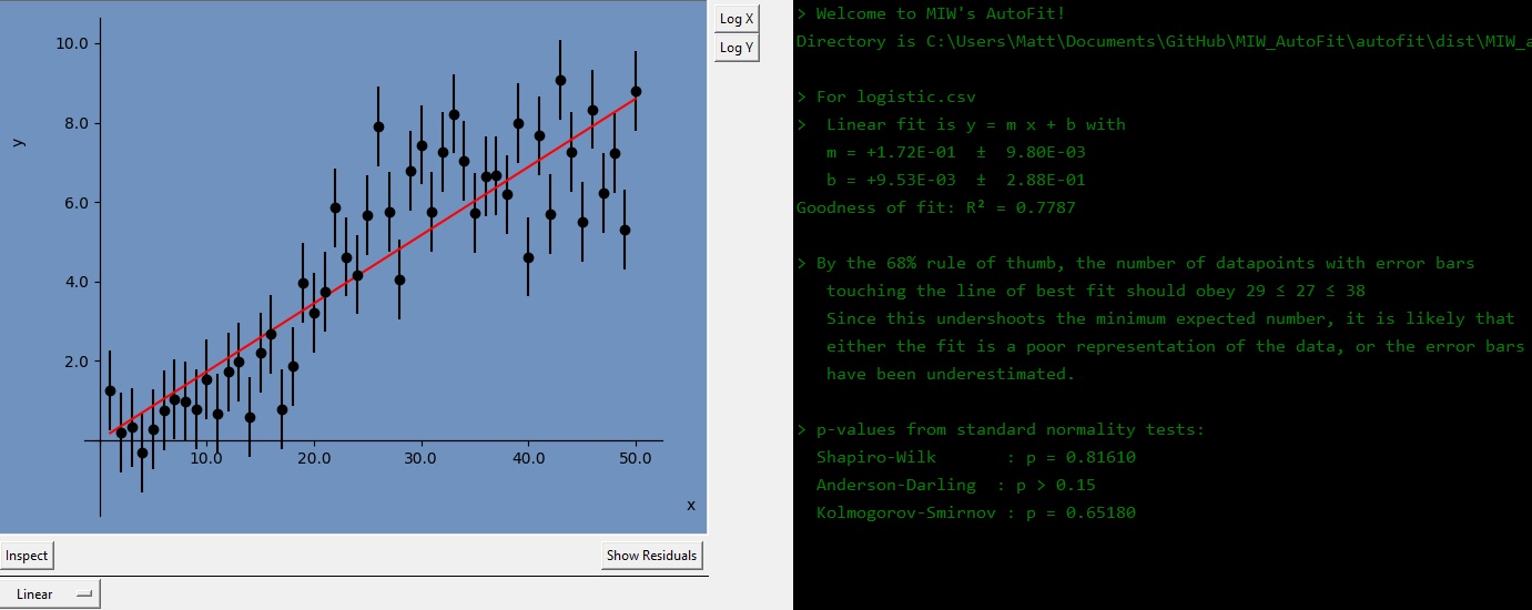
Let’s make sure AutoFit has a fresh start so we’re all on the same page. After closing the window, open AutoFit again and load up logistic.csv⭳ . When we fit the data, it looks decent enough, but if you care to look at the residuals, at least one of the measures on the console will tell you that the fit isn’t quite right, meaning the data might have features which are not reflected in the linear model we have chosen.

Now let’s try to find a better model from the quick options. Hover over the dropdown menu currently called Linear. It will show a list of options, and for now let’s choose Polynomial.

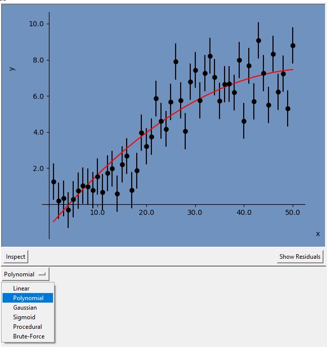
The default polynomial will be of order two (i.e. a quadratic equation). The arrows which have appeared below the dropdown handle will allow you to choose the degree. You can go as low as 0, and up to one less than the number of data points you have.

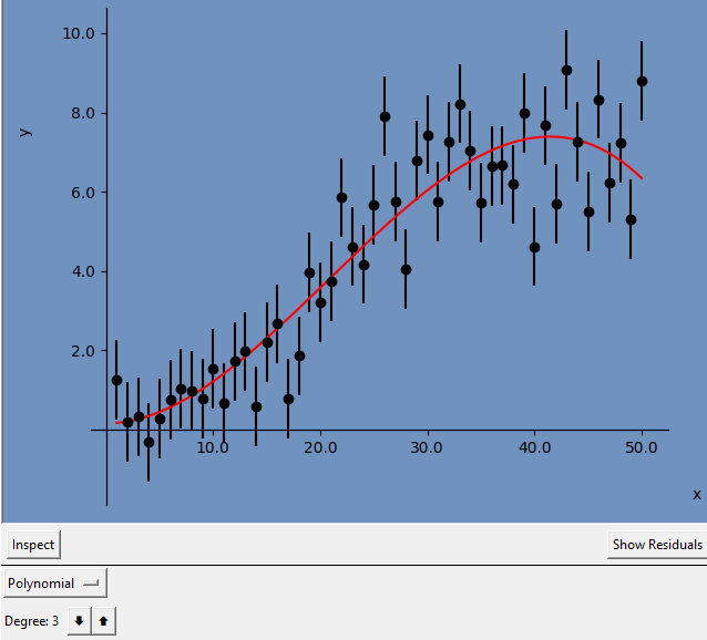
You can play around with it to find the fit that suits you best. Personally I like the 3rd degree fit. After a certain point (for me degree 15) the uncertainties become NaN (not a number) meaning the algorithm isn’t stable, and which I interpret as the fit losing statistical meaning.

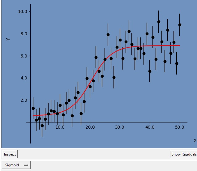
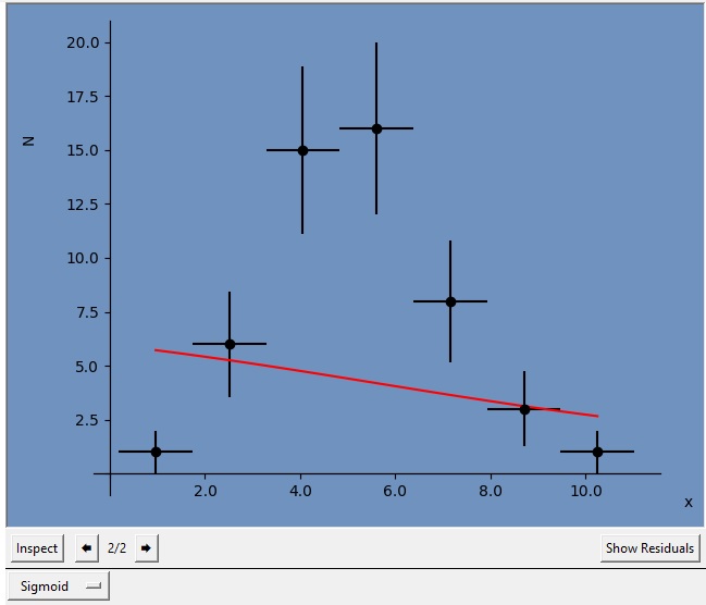
Now let’s try another dropdown, this time picking Sigmoid. The sigmoid function here is defined as

which you should also be able to see in the console area.

Next let’s do something a bit different. Load in random sample from normal_distribution.csv⭳ . This is just a list of numbers, but AutoFit will find an appropriate bin size to make a nice histogram of the data.

The fit line will look terrible since we’re still on Sigmoid. If you’re used to Gaussian functions or Normal distributions, try estimating by eye the mean and the standard deviation of the sample before moving on to the next step.

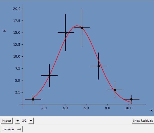
Now change the fit-type dropdown list to Gaussian. You should get a beautiful fit, showing a mean of 5 and a standard deviation of 2, give or take.

Since this is a histogram, you might want to normalize the histogram to show probabilities instead. On the right side of the image, you can press Normalize to set the integral over all bins to 1.

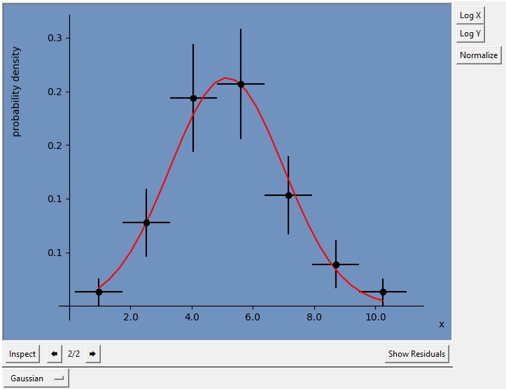
Since AutoFit knows the histogram has been normalized, you might also notice that the console displays a different function with different fit estimates, corresponding to the Normal distribution rather than a Gaussian.

In the next tutorial, we take a look at finding the best model when we don’t know in the first place which model should fit!