
MIWs AutoFit – Tutorial 1 – Getting Started
Published:
In this tutorial we open and fit .csv and .xls data to a linear model, learn how AutoFit displays parameter estimates and uncertainties, see how to analyze multiple datasets at once, and discover the residuals button.
Welcome to MIW’s AutoFit! I prefer to teach by doing rather than by listing a bunch of things that are possible, so let’s open up AutoFit to get started.
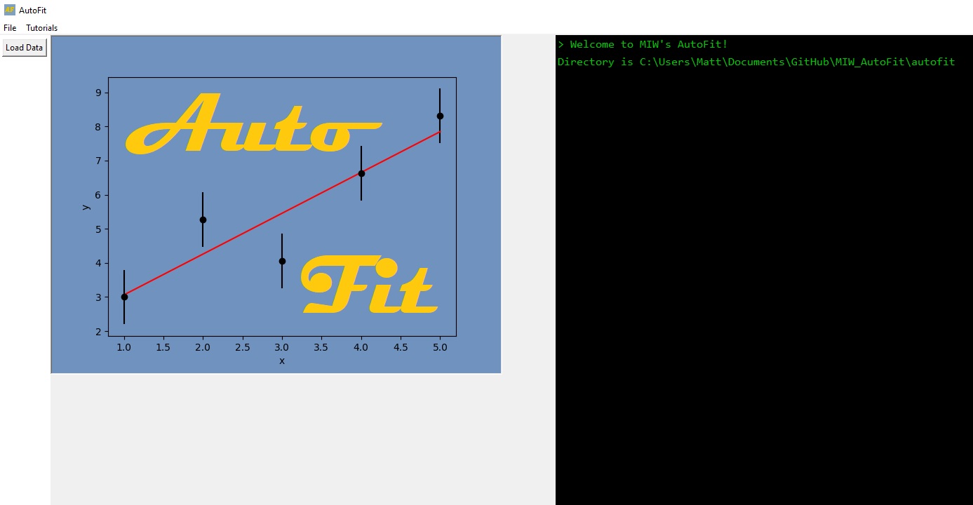
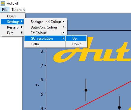
The text might be too large or small for your taste, so use the file menu to adjust the font size. The image panel can be resized using your mouse’s scroll wheel. You can also try right-clicking on the image or the console area if you don’t like the colour scheme.
Now let’s load up a dataset. The package should come with all the sample sets used in this tutorial, but if you can’t find it, we will also provide the files in these tutorial pages. Let’s click load data and navigate to linear_data_yerrors.csv⭳ .
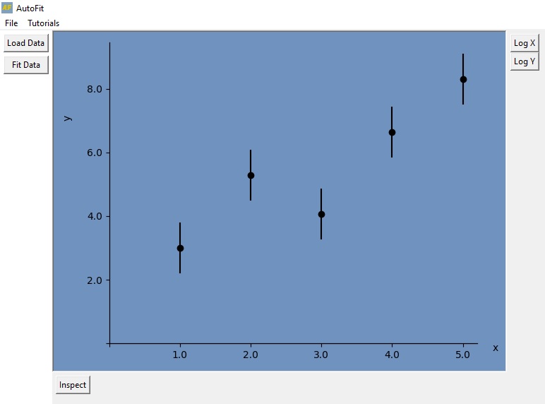
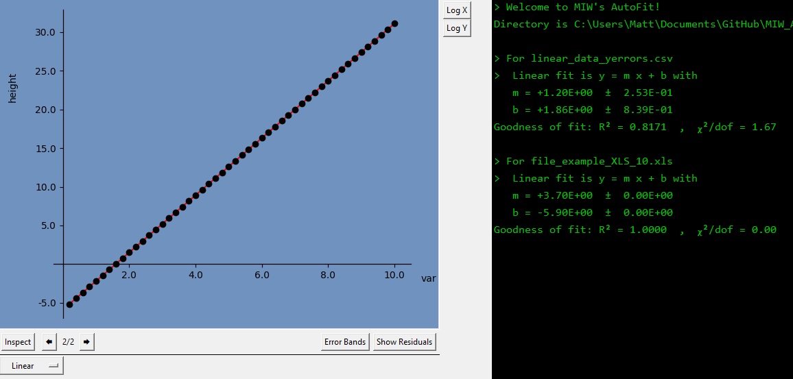
Some new options have appeared. You can log the data in the x- and y- coordinates, which can be useful when data spans many orders of magnitude. You can also inspect the plot, which will make a window pop out allowing you to zoom in on certain features, and can let you save the plot on your filesystem. What we’ll do next though is fit the data with the new “Fit Data” button on the left.
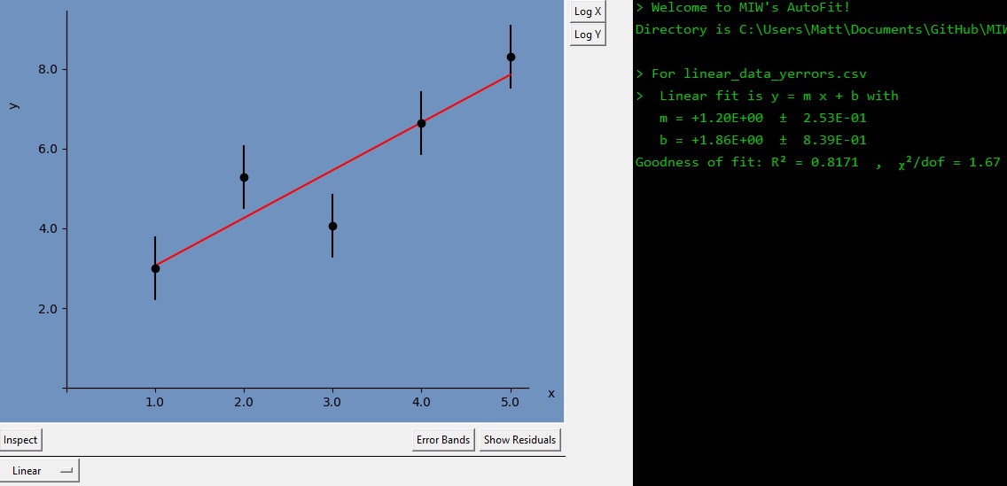
Look at that, you’ve reproduced the plot for the splash screen! The console-esque output on the right shows you the parameters of your fit, along with their uncertainties. As in most physics applications, the quoted uncertainty after the ± symbol is the standard deviation of the mean. For more details about the methods used to find fits and uncertainties, you can view the references page.
Let’s say you also have another linear dataset you want to plot. Click load data and select file example_XLS_10.xls⭳
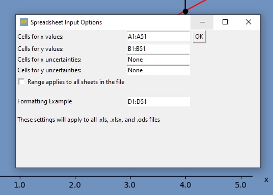
The x-data in this file is between A1 and A51, while the y-data is between B1 and B51. Put a colon : between the start and end values to tell AutoFit what the data range is.
Also note that if your excel file has multiple sheets – where the data is in the same place in each – you can click the tick box to load in the data from every sheet.
The new data appears, with the dataset automatically fit using the current model. You can use the new arrow buttons below the image to switch between loaded datasets.
If you would like to compare both datasets, you can press the Fit All button on the left. All loaded datasets will be overlayed, with the average fit being displayed in red.
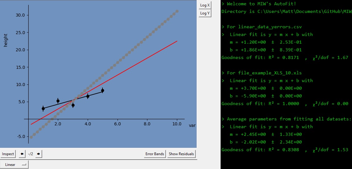
The console panel on the far right will display the best fit parameters and uncertainty estimates for this average fit.
Finally, let’s load up one more dataset to showcase the Show Residuals button. Opening and fitting linear_data_multiple_measurements.csv⭳ , we see that multiple measurements have been made at each x-value. Now click Show Residuals.
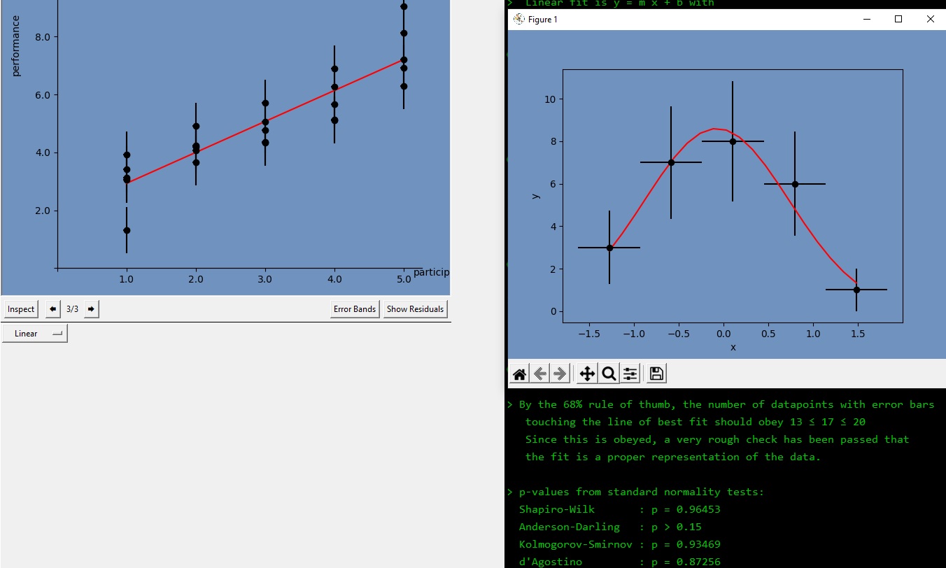
Residuals are defined as \(r_i = y_i - f(x_i)\). For well-fit data, residuals should follow a Gaussian distribution. The residuals are binned into a histogram, and the fit to a Gaussian is overlayed.
The details provided in the console area give information on how well the residuals conform to a normal distribution. As a rule of thumb, if the standard tests for normality show a p-value of p < 0.05, you have some evidence that your line of best fit is not an appropriate model for the data. If the standard tests disagree with one another, you will have to use your own judgement based on the collective information provided.
In the next tutorial, we take a look at fitting with other commonly-used functional models.